In part 1, we laid the groundwork for our Reinforcement Learning experiments by creating a simple game (Swoggle) that we’d be trying to teach out AI to play. We also created some simple Agents that followed hard-coded rules for play, to give our AI some opponents. In this post, we’ll get to the hard part – using RL to learn to play this game.
The Task
Reinforcement Learning (Artist’s Depiction)
We want to create some sort of Agent capable of looking at the state of the game and deciding on the best move. It should be able to learn the rules and how to win by playing many games. Concretely, our agent should take in an array encoding the dice roll, the positions of the players and bases etc, and it should output one of 192 possible moves (64 squares, with two special kinds of move to give 64*3 possible actions). This agent shouldn’t just be a passive actor – it must also be able to learn from past games.
Policy Networks
In RL, a ‘policy’ is a map from game state to action. So when we talk about ‘Policy Learners’, ‘Policy Gradients’ or ‘Policy Networks’, we’re referring to something that is able to learn a good policy over time.
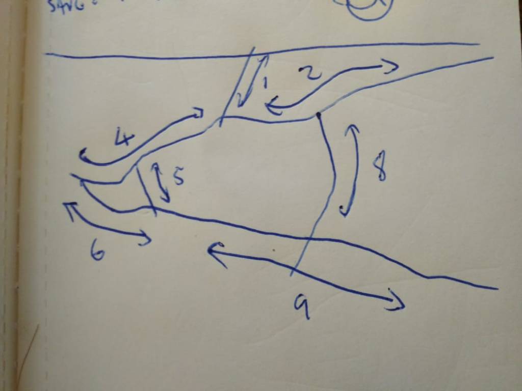
The network we’ll be training
So how would we ‘learn’ a policy? If we had a vast archive of past games, we could treat this as a supervised learning task – feed in the game state, chosen action and eventual reward for each action in the game history to a neural network or other learning algorithm and hope that it learns what ‘good’ actions look like. Sadly, we don’t have such an archive! So, we take the following approach:
Start a game (an ‘episode’)
Feed the game state through our policy network, which initially will give random output probabilities on each possible action
Pick an action, favoring those for which the network output is high
Keep making actions and feeding the resultant game state through the network to pick the next one, until the game ends.
Calculate the reward. If we won, +100. If we lost, -20. Maybe an extra +0.1 for each valid move made, and some negative reward for each time we tried to break the rules.
Update the network, so that it (hopefully) will better predict which moves will result in positive rewards.
Start another game and repeat, for as long as you want.
The initial example (like most resources you’ll find if you look around) chooses a problem with a single action – up or down, for example. I modified the network to take in 585 inputs (the Swoggle game state representation) and give out 192 outputs for the 62*3 possible actions an agent could take. I also added the final sigmoid layer since I’ll be interpreting the outputs as probabilities.
Many implementations either take random actions (totally random) or look at the argmax of the network output. This isn’t great in our case – random actions are quite often invalid moves, but the top output of the network might also be invalid. Instead, we sample an action from the probability distribution represented by the network output. This is like the approach Andrej Karpathy takes in his classic ‘Pong from Pixels’ post (which I highly recommend).
This game is dice-based (which adds randomness) and not all actions are possible at all times, so I needed to add code to handle cases where the proposed move is invalid. In those cases, we add a small negative reward and try a different action.
The implementation I started from used a parameter epsilon to shift from exploration (making random moves) to optimal play (picking the top network output). I removed this – by sampling from the prob. distribution, we keep our agent on it’s toes, and it always has a chance of acting randomly/unpredictably. This should make it more fun to play against, while still keeping it’s ability to play well most of the time.
This whole approach takes a little bit of time to internalize, and I’m not best placed to explain it well. Check out the aforementioned ‘Pong from Pixels’ post and google for Policy Gradients to learn more.
Early on, I seemed to have hit upon an excellent strategy. Within a few games, my Agent was winning nearly 50% of games against the basic game AI (for a four player game, anything above 25% is great!). Digging a little deeper, I found my mistake. If the agent proposed a move that was invalid, it stayed where it was while the other agents moved around. This let it ‘camp’ on it’s base, or wait for a good dice roll before swoggling another base. I was able to get a similar win-rate with the following algorithm:
Pick a random move
If it’s valid, make the move. If not, stay put (not always a valid action but I gave the agent control of the board!)
That’s it – that’s the ‘CheatyAgent’ algorithm 🙂 Fortunately, I’m not the first to have flaws in my game engine exploited by RL agents – check out the clip from OpenAI above!
Another bug: See where I wrote sr.dice() instead of dice_roll? This let the network re-roll if it proposed an invalid move, which could lead to artificially high performance.
After a few more sneaky attempts by the AI to get around my rules, I finally got a setup that forced the AI to play by the rules, make valid moves and generally behave like a good and proper Swoggler should.
Winning for real
Learning to win!!!
With the bugs ironed out, I could start tweaking rewards and training the network! It took a few goes, but I was able to find a setup that let the agent learn to play in a remarkably short time. After a few thousand games, we end up with a network that can win against three BasicAgents about 40-45% of the time! I used the trained network to pick moves in 4000 games, and it won 1856 of them, confirming it’s superiority to the BasicAgents, who hung their heads in shame.
So much more to try
I’ve still got plenty to play around with. The network still tries to propose lots of invalid moves. Tweaking the rewards can change this (note the orange curve below that tracks ratio of valid:invalid moves) but at the cost of diverting the network from the true goal: winning games!
Learning to make valid moves, but at the cost of winning.
That said, I’m happy enough with the current state of things to share this blog. Give it a go yourself! I’ll probably keep playing with this, but unless I find something super interesting, there probably won’t be a part 3 in this series. Thanks for coming along on my RL journey 🙂
I’m going to be exploring the world of Reinforcement Learning. But there will be no actual RL in this post – that’s for part two. This post will do two things: describe the game we’ll be training our AI on, and show how I developed it using a tool called NBDev which is making me so happy at the moment. Let’s start with NBDev.
What is NBDev?
Like many, I started my programming journey editing scripts in Notepad. Then I discovered the joy of IDEs with syntax highlighting, and life got better. I tried many editors over the years, benefiting from better debugging, code completion, stylish themes… But essentially, they all offer the same workflow: write code in an editor, run it and see what happens, make some changes, repeat. Then came Jupyter notebooks. Inline figures and explanations. Interactivity! Suddenly you don’t need to re-run everything just to try something new. You can work in stages, seeing the output of each stage before coding the next step. For some tasks, this is a major improvement. I found myself using them more and more, especially as I drifted into Data Science.
But what about when you want to deploy code? Until recently, my approach was to experiment in Jupyter, and then copy and paste code into a separate file or files which would become my library or application. This caused some friction – which is where NBDev comes in.
With NBDev, everything happens in your notebooks. By adding special comments like #export to the start of a cell, you tell NBDev how to treat the code. This means you can write a function that will be exported, write some examples to illustrate how it works, plot the results and surround it with nice explanations in markdown. The exported code gets paces in a neat, well-ordered .py file that becomes your final product. The Notebook(s) becomes documentation, and the extra examples you added to show functionality work as tests (although you can also add more formal unit testing). An extra line of code uploads your library for others to install with pip. And if you’re following their guide, you get a documentation site and continuous integration that updates whenever you push your changes to GitHub.
The upshot of all this is that you can effortlessly create good, clean code and documentation without having to switch between notebooks, editors and separate documentation. And the process you followed, the journey that lead to the final design choices, is no longer hidden. You can show how things developed, and include experiments that justify a particular choice. This is ‘literate programming’, and it feels like a major shift in the way I think about software development. I could wax lyrical about this for ages, but you should just go and read about it in the launch post here.
What on Earth is Swoggle?
Christmas, 2019. Our wedding has brought a higher-than-normal influx of relatives to Cape Town, and when this extended family gets together, there are some things that are inevitable. One of these, it turns out, is the invention of new games to keep the cousins entertained. And thus, Swoggle was born 🙂
A Swoggle game in progress – 2 players are left.
The game is played on an 8×8 board. There are usually 4 players, each with a base in one of the corners. Players can move (a dice determines how far), “spoggle” other players (capturing them and placing them in “swoggle spa” – none of this violent termnology) or ‘swoggle’ a base (gently retiring the bases owner from the game – no killing here). To make things interesting, there are four ‘drones’ that can be used as shields or to take an occupied base. Moving with a drone halves the distance you can travel, to make up for the advantages. A player with a drone can’t be spoggled by another player unless they too have a drone, or they ‘powerjump’ from their base (a half-distance move) onto the droned player. Maybe I’ll make a video one day and explain the rules properly 🙂
So, that’s the game. Each round is fairly quick, so we usually play multiple rounds, awarding points for different achievements. Spoggling (capturing) a player: 1 point. Swoggling (taking out a base): 3 points. Last one standing: 5 points. The dice rolls add lots of randomness, but there is still plenty of room for tactics, sibling rivalry and comedic mistakes.
Game Representation
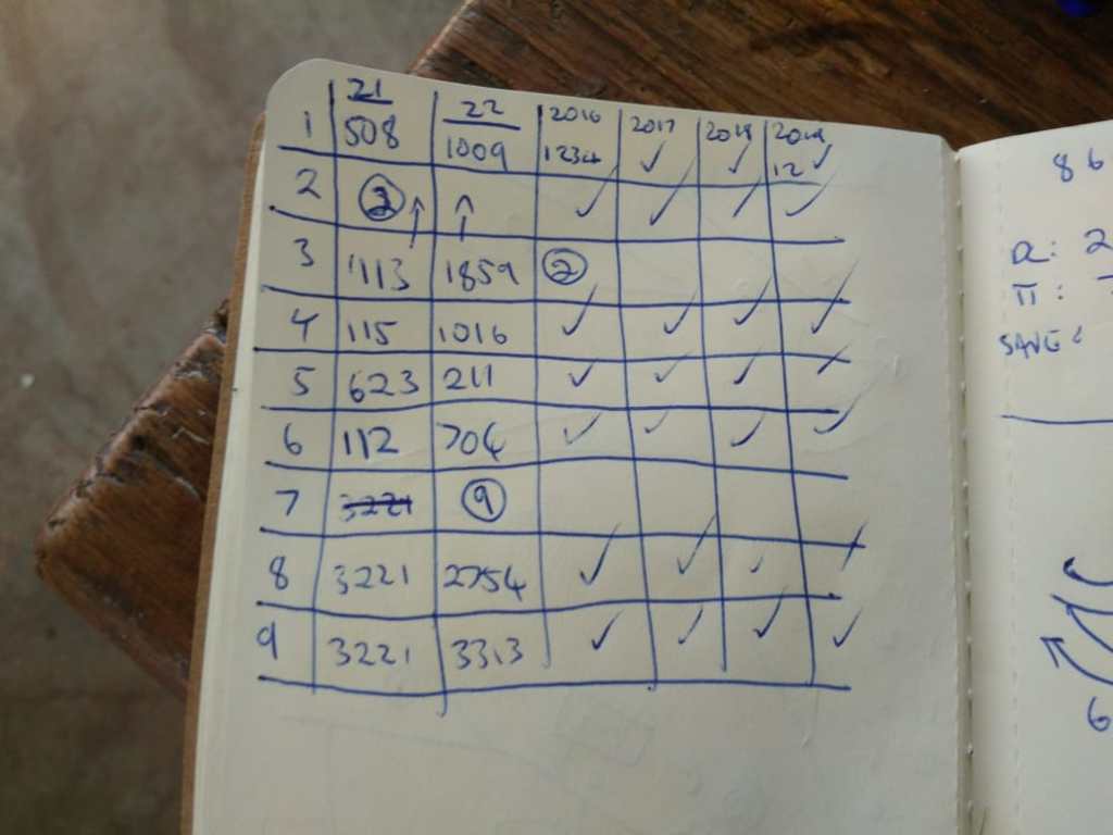
If we’re going to teach a computer to play this, we need a way to represent the game state, check if moves are valid, keep track of who’s in the swoggle spa and which bases are still standing, etc. I settled on something like this:
Game state representation
There is a Cell in each x, y location, with attributes for player, drone and base. These cells are grouped in a Board, which represents the game grid and tracks the spa. The Board class also contains some useful methods like is_valid_move() and ways to move a particular player around. At the highest level, I have a Swoggle class that wraps a board, handles setting up the initial layout, provides a few extra convenience functions and can be used to run a game manually or with some combination of agents (which we’ll cover in the next section). Since I’m working in NBDev, I have some docs with almost no effort, so check out https://johnowhitaker.github.io/swoggle/ for details on this implementation. Here’s what the documentation system turned my notebooks into:
Part of the generated documentation
The ability to write code and comments in a notebook, and have that turn into a swanky docs page, is borderline magical. Mine is a little messy since this is a quick hobby project. To see what this looks like in a real project, check out the docs for NBDev itself or Fastai v2.
Creating Agents
Since the end goal is to use this for reinforcement learning, it would be nice to have an easy way to add ‘Agents’ – code that defines how a player in the game will make a move in a given situation. It would also be useful to have a few non-RL agents to test things out and, later, to act as opponents for my fancier bots. I implemented two types of agent:
RandomAgent Simply picks a random but valid move by trial and error, and makes that move.
BasicAgent Adds a few simple heuristics. If it can take a base, it does so. If it can spoggle a player, it does so. If neither of these options are possible, it moves randomly.
You can see the agent code here. The notebook also defines a few other useful functions, such as win_rates() to pit different agents against each-other and see how they do. This is fun to play with – after a few experiments it’s obvious that the board layout and order of players matters a lot. A BasicAgent going last will win ~62% of games against three RandomAgents – not unexpected. But of the three RandomAgents, the one opposite the BasicAgent (and thus furthest from it) will win the majority of the remaining games.
Next Step: Reinforcement Learning!
This was a fun little holiday coding exercise. I’m definitely an NBDev convert – I feel so much more productive using this compared to any other development approach I’ve tried. Thank you Jeremy, Sylvain and co for this excellent tool!
Now, the main point of this wasn’t just to get the game working – it was to use it for something interesting. And that, I hope, is coming soon in Part 2. As I type this, a neural network is slowly but surely learning to follow the rules and figuring out how to beat those sneaky RandomAgents. Wish it luck, stay tuned, and, if you’re *really* bored, pip install swoggle and watch some BasicAgents battle it out 🙂
Ever wondered what goes into launching a data science competition? If so, this post is for you. I spent the last few days working on the Fowl Escapades: Southern African Bird Call Audio Identification Challenge on Zindi, and thought it would be fun to take you behind the scenes a little to show how it all came together.
Step 1: Inspiration
Many competitions spring from an existing problem in need of a solution. For example, you may want a way to predict when your delivery will arrive based on weather, traffic conditions and the route your driver will take. In cases like this, an organization will reach out to Zindi with this problem statement, and move to stage 2 to see if it’s a viable competition idea. But this isn’t the only way competitions are born!
Sometimes, we find a cool dataset that naturally lends itself to answering an interesting problem. Sometimes we start with an interesting problem, and go looking for data that could help find answers. And occasionally, we start with nothing but a passing question at the end of a meeting: ‘does anyone have any other competition ideas?’. This was the case here.
I had been wanting to try my hand at something involving audio data. Since I happen to be an avid birder, I thought automatic birdsong identification would be an interesting topic. For this to work, we’d need bird calls – lot’s of them. Fortunately, after a bit of searching I found the star of this competition: https://www.xeno-canto.org/. Hundreds of thousands of calls from all over the world! A competition idea was born.
Step 2: Show me the data
To run a competition, you need some data (unless you’re going to ask the participants to find it for themselves!). This must:
Be shareable. Anything confidential needs to be masked or removed, and you either need to own the data or have permission to use it. For the birdsong challenge, we used data that had CC licences but we still made sure to get permission from xeno-canto and check that we’re following all the licence terms (such as attribution and non-modification).
Be readable. This means no proprietary formats, variable definitions, sensible column names, and ideally a guide for reading in the data.
Be manageable. Some datasets are HUGE! It’s possible to organize contests around big datasets, but it’s worth thinking about how you expect participants to interact with the data. Remember – not everyone has fast internet or free storage.
Be useful. This isn’t always easy to judge, which is why doing data exploration and building a baseline model early on is important. But ideally, the data has some predictive power for the thing you’re trying to model!
Visualizing birdsongs
By the time a dataset is released as part of a competition, it’s usually been through several stages of preparation. Let’s use the birdsong example and look at a few of there steps.
Collection: For an organization, this would be an ongoing process. In our example case, this meant scraping the website for files that met our criteria (Southern African birds) and then downloading tens of thousands of mp3 files.
Cleaning: A catch-all term for getting the data into a more usable form. This could be removing unnecessary data, getting rid of corrupted files, combining data from different sources…
Splitting and Masking: We picked the top 40 species with the most example calls, and then split the files for each species into train and test sets, with 33% of the data kept for the test set. Since the file names often showed the bird name, we used ''.join(random.choices(string.ascii_uppercase + string.digits, k=6)) to generate random IDs. However you approach things, you’ll need to make sure that the answers aren’t deducible from the way you organize things (no sorting by bird species for the test set!)
Checking(and re-checking, and re-checking): Making sure everything is in order before launch is vital – nothing is worse than trying to fix a problem with the data after people have started working on your competition! In the checking process I discovered that some mp3s had failed to download properly, and others were actually .wav files with .mp3 as the name. Luckily, I noticed this in time and could code up a fix before we went live.
Many of these steps are the same when approaching a data science project for your own work. It’s still important to clean and check the data before launching into the modelling process, and masking is useful if you’ll need to share results or experiments without necessarily sharing all your secret info.
Step 3: Getting ready for launch
Aside from getting the data ready, there are all sorts of extra little steps required to arrive at something you’re happy to share with the world. An incomplete list of TODOs for our latest launch:
Decide on a scoring metric. This will be informed by the type of problem you’re giving to participants. In this case, we were torn between accuracy and log loss, and ended up going with the latter. For other cases (eg imbalanced data), there are a host of metrics. Here’s a guide: https://machinelearningmastery.com/tour-of-evaluation-metrics-for-imbalanced-classification/
Put together an introduction and data description. What problem are we solving? What does the solution need to do? What does the training data look like? This will likely involve making some visualizations, doing a bit of research, finding some cool images to go with your topic…
Social media. This isn’t part of my job, but I gather that there is all sorts of planning for how to let people know about the cool new thing we’re putting out into the world 🙂
Tutorials. Not essential, but I feel that giving participants a way to get started lowers the barriers to entry and helps to get more novices into the field. Which is why, as is becoming my habit, I put together a starter notebook to share as soon as the contest launches.
A confusion matrix – one way to quickly see how well a classification algorithm is working. (from the starter notebook)
Baseline/benchmark. This is something I like to do as early as possible in the process. I’ll grab the data, do the minimal cleaning required, run it through some of my favorite models and see how things go. This is nice in that it gives us an idea of what a ‘good’ score is, and whether the challenge is even doable. When a client is involved, this is especially useful for convincing them that a competition is a good idea – if I can get something that’s almost good enough, imagine what hundreds of people working for prize money will come up with! If there’s interest in my approach for a quick baseline, let me know and I may do a post about it.
Names, cover images, did you check the data???, looking at cool birds, teaser posts on twitter, frantic scrambles to upload files on bad internet, overlaying a sonogram on one of my bird photos… All sorts of fun 🙂
Fine-tuning the benchmark model
I could add lots more. I’ve worked on quite a few contests with the Zindi team, but usually I’m just part of the data cleaning and modelling steps. I’ve had such a ball moving this one from start to finish alongside the rest of the team, and I really appreciate all the hard work they do to keep us DS peeps entertained!
Try it yourself!
I hope this has been interesting. As I said, this whole process has been a blast. So if you’re sitting on some data, or know of a cool dataset, why not reach out and host a competition? You might even convince them to let you name it something almost as fun as ‘Fowl Escapades’. 🙂
Driven Data launched a competition around the Snapshot Serengeti database – something I’ve been intending to investigate for a while. Although the competition is called “Hakuna Ma-data” (which where I come from means something like “there is no data”), this is actually the largest dataset I’ve worked with to date, with ~5TB of high-res images. I suspect that that’s putting people off (there are only a few names on the leaderboard), so I’m writing this post to show how I did an entry, run through some tricks for dealing with big datasets, give you a notebook to get started quickly and try out a fun new tool I’ve found for monitoring long-running experiments using neptune.ml.Let’s dive in.
The Challenge
The goal of the competition is to create a model that can correctly label the animal(s) in an image sequence from one of many camera traps scattered around the Serengeti plains, which are teeming with wildlife. You can read more about the data and the history of the project on their website. There can be more than one type of animal in an image, making this a multi-label classification problem.
Some not-so-clear images from the dataset
The drivendata competition is interesting in that you aren’t submitting predictions. Instead, you have to submit everything needed to perform inference in their hidden test environment. In other words, you have to submit a trained model and the code to make it go. This is a good way to practice model deployment.
Modelling
The approach I took to modelling is very similar to the other fastai projects I’ve done recently. Get a pre-trained resnet50 model, tune the head, unfreeze, fine-tune, and optionally re-train with larger images right at the end. It’s a multi-label classification problem, so I followed the fastai planet labs example for labeling the data. You can see the details of the code in the notebook (coming in the next section) but I’m not going to go over it all again here. The modelling in this case is less interesting than the extra things needed to work at this scale.
Starter Notebook
I’m a big fan of making data science and ML more accessible. For anyone intimidated by the scale of this contest, and not too keen on following the path I took in the rest of this post, I’ve created a Google Colab Notebook to get you started. It shows how to get some of the data, label it, create and train a model, score your model like they do in the competition and create a submission. This should help you get started, and will give a good score without modification. The notebook also has some obvious improvements waiting to be made – using more data, training the model further…..
Training a quick model in the starter notebook
The code in the notebook is essentially what I used for my first submission, which is currently the top out of the… 2 total submissions on the leaderboard. As much as I like looking good, I’ll be much happier if this helps a bunch of people jump ahead of that score! Please let me know if you use this, so that I don’t feel that this wasn’t useful to anyone?
Moar Data – Colab won’t cut it
OK, so there definitely isn’t 5TB of storage on Google Colab, and even though we can get a decent score with a fraction of the data, what if we want to go further? My approach was as follows:
Create a Google Cloud Compute instance with all the fastai libraries etc installed, by following this tutorial. The resultant machine has 50GB memory, a P100 GPU and 200GB disk space by default. It comes with most of what’s required for deep learning work, and has the added bonus of having jupyter + all the fastai course notebooks ready to get things going quickly. I made sure not to make the instance preemptible – we want to have long-running tasks going, so having it shut down unexpectedly would be sad.
Add an extra disk to the compute instance. This tutorial gave me the main steps. It was quite surreal typing in 6000 GB for the size! I mounted the dist at /ss_ims – that will be my base folder going forward.
Download a season of data, and then begin experimenting while more downloads. No point having that pricey GPU sitting idle!
Train the full model overnight, tracking progress.
Submit!
Mounting a scarily large disk!
I won’t go into the cloud setup here, but in the next section let’s look at how you can track the status of a long-running experiment.
Neptune ML – Tracking progress
I’d set the experiments running on my cloud machine, but due to lack of electricity and occasional loss of connection I couldn’t simply leave my laptop running and connected to the VM to show how the model training was progressing. With so many images, each epoch of training took ages, and I had a couple of models crash early in the process. This was frustrating – I would try to leave it going overnight but if the model failed in the evening it meant that I had wasted some of my few remaining cloud credits on a machine sitting idle. Luckily, I had recently seen how to monitor progress remotely, meaning I could check my phone while I was out and see if the model was working and how good it was getting.
Tracking loss and metrics over time with neptune.ml
The process is pretty simple, and well documented here. You sign up for an account, get an API key and add a callback to your model. This will then let you log in to neptune.ml from any device, and track your loss, any metrics you’ve added and the output of the code you’re running. I could give more reasons why this is useful, but honestly the main motivation is that it’s cool! I had great fun surreptitiously checking my loss from my phone every half hour while I was out and about.
Tracking model training with neptune
Where next?
I’m out of cloud credits, and as an ‘independent scientist’ my funding situation doesn’t really justify spending more money on cloud compute to try a better entry. If you’d like to sponsor some more work, I may have another go with a properly trained model. I did manage to experiment on using more than the first image in a sequence, and using Jeremy Howard’s trick of doing some final fine-tuning on larger images – would be interesting to see how much these improve the score in this contest.
I hope this post encourages more of you to try this contest out! As the starter notebook shows, you can get close to the top (beating the benchmark) with a tiny fraction of the data and some simple tricks. Give it a try and report how you do in the comments!
Every now and again, the World Bank conducts something called a Living Standards Measurement Study (LSMS) survey in different countries, with the purpose being to learn about people, their incomes and expenses, how they’re doing economically and so on. These surveys provide very useful info to various stakeholders, but they’re expensive to conduct. What if we could estimate some of the parameters they measure from satellite imagery instead? That was the goal of some researchers at Stanford back in 2016, who came up with a way to do just that and wrote it up into this wonderful paper in Science. In this blog post, we’ll explore their approach, replicate the paper (using some more modern tools) and try a few experiments of our own.
Predicting Poverty: Where do you start?
Nighttime lights
How would you use remote sensing to estimate economic activity for a given location? One popular method is to look at how much light is being emitted there at night – as my 3 regular readers may remember, there is a great nighttime lights dataset produced by NOAA that was featured in a data glimpse a while back. It turns out that the amount of light sent out does correlate with metrics such as assets and consumption, and this data has been used in the past to model things like economic activity (see another data glimpse post for more that). One problem with this approach: the low end of the scale gets tricky – nighttime lights don’t vary much below a certain level of expenditure.
Looking at daytime imagery, we see many things that might help tell us about the wealth in a place: type of roofing material on the houses, the number of roads, how built-up an area is…. But there’s a problem here too: these features are quite complicated, and training data is sparse. We could try to train a deep learning model to take in imagery and spit out income level, but the LSMS surveys typically only cover a few hundred locations – not a very large dataset, in other words.
Jean et al’s sneaky trick
The key insight in the paper is that we can train a CNN to predict nighttime lights (for which we have plentiful data) from satellite imagery, and in the process it will learn features that are important for predicting lights – and that these features will likely also be good for predicting our target variable as well! This multi-step transfer learning approach did very well, and is a technique that’s definitely worth keeping in mind when you’re facing a problem without much data.
The authors of the paper shared their code publicly but… it’s a little hard to follow, and is scattered across multiple R and Python files. Luckily, someone has already done some of the hard work for us, and has shared a pytorch version in this GitHub repository. If you’d like to replicate the paper exactly, that’s a good place to start. I’ve gone a step further and consolidated everything into a single Google Colab notebook that borrows code from the above and builds on it. The rest of this post will explain the different sections of the notebook, and why I depart from the exact method used in the paper. Spoiler: we get a slightly better result with much fewer images downloaded.
Getting the data
The data comes from the Fourth Integrated Household Survey 2016-2017. We’ll focus on Malawi for this post. The notebook shows how to read in several of the CSV files downloaded from the website, and combine them into ‘clusters’ – see below. For each cluster location, we have a unique ID (HHID), a location (lat and lon), an urban/rural indicator, a weighting for statisticians, and the important variable: consumption (cons). This last one is the thing we’ll be trying to predict.
The relevant info from the survey data
One snag: the lat and lon columns are tricksy! They’ve been shifted to protect anonymity, so we’ll have to consider a 10km buffer around the given location and hope the true location is close enough that we get useful info.
Adding nighttime lights
Getting the nightlights value for a given location
To get the nightlight data, we’ll use the python library to run Google Earth Engine queries. You’ll need a GEE account, and the notebook shows how to authenticate and get the required data. We can get the nightlights for each cluster location (getting the mean over an 8km buffer around the lat/lon points) and add this number as a column. To give us a target to aim at, we’ll compare any future models to a simple model based on these nightlight values only.
Downloading static maps images
Getting imagery for a given location
The next step takes a while: we need to download images for the locations. BUT: we don’t just want one for each cluster location – instead, we want a selection from the surrounding area. Each of these will have it’s own nightlights value, so that we get a larger training set to build our model on. Later, we’ll extract features for each image in a cluster and combine them. Details are in the notebook. The code takes several hours to run, but at the end of it you’ll have thousands of images ready to use.
Tracking requests/sec on in my Google Cloud Console
You’ll notice that I only generate 20 locations around each cluster. The original paper uses 100. Reasons: 1) I’m impatient. 2) There is a rate limit of 25k images/day, and I didn’t want to wait (see #1), 3) The images are 400 x 400, but are then shrunk to train the model. I figured I could split the 400px image into 4 (or 9) smaller images that overlap slightly, and thus get more training data for free. This is suggested as a “TO TRY” in the notebook, but hint: it works. If you really wanted to get a better score, trying this or adding more imagery is an easy way to do so.
Training a model
I’ll be using fastai to simplify the model creation and training stages. before we can create a model, we need an appropriate databunch to hold the training data. An optional addition at this stage is to add image transforms to augment our training data – which I do with tfms = get_transforms(flip_vert=True, max_lighting=0.1, max_zoom=1.05, max_warp=0.) as suggested in the fastai satelite imagery example based on Planet labs. The notebook has the full code for creating the databunch:
Data ready for modelling
Next, we choose a pre-trained model and re-train it with our data. Remember, the hope is that the model will learn features that are related to night lights and, by extension, consumption. I’ve had decent results with resnet models, but in the shared notebook I stick with models.vgg11_bn to more closely match the original paper. You could do much more on this model training step, but we pick a learning rate, train for a few epochs and move on. Another place to improve!
Training the model to predict nightlights
Using the model as a feature extractor
This is a really cool trick. We’ll hook into one of the final layers of the network, with 512 outputs. We’ll save these outputs as each image is run through the network, and they’ll be used in later modelling stages. To save the features, you could remove the last few layers and run the data through, or you can use a trick I learnt from this TDS article and keep the network intact.
Cumulative explained variance of top PCA features
512 (or 4096, depending on the mode and which layer you pick) is a lot of features. So we use PCA to get 30 or so meaningful features from those 512 values. As you can see from the plot above, the top few components explain most of the variance in the data. These top 30 PCA components are the features we’ll use for the last step in the process: predicting consumption.
Putting it all together
For each image, we now have a set of 30 features that should be meaningful for predicting consumption. We group the images by cluster (aggregating their features). Now, for each cluster, we have the target variable (‘cons’), the nighttime lights (‘nl’) and 30 other potentially useful features. As we did right at the start, we’ll split the data into a test and a train set, train a model and then make predictions to see how well it does. Remember: our goal is to be better than a model that just uses nighttime lights. We’ll use the r^2 score when predicting log(y), as in the paper. The results:
Score using just nightlights (baseline): 0.33
Score with features extracted from imagery: 0.41
Using just the features derived from the imagery, we got a significant score increase. We’ve successfully used deep learning to squeeze some useful information out of satellite imagery, and in the process found a way to get better predictions of survey outcomes such as consumption. The paper got a score of 0.42 for Malawi using 100 images to our 20, so I’d call this a success.
Improvements
There are quite a few ways you can improve the score. Some are left as exercises for the reader 🙂 here are a few that I’ve tried: 1) Tweaking the model used in the final step: 0.44 (better than the paper) 2) Using sub-sampling to boost size of training dataset + using a random forest model: 0.51 (!) 3) Using a model trained for classification on binned NL values (as in paper) as opposed to training it on a regression task: score got worse 4) Cropping the downloaded images into 4 to get more training data for the model (no other changes): 0.44 up from 0.41 without this step. >0.5 aggregating features of 3 different subsets of images for each cluster 5) Using a resnet-50 model: 0.4 (no obvious change this time – score likely depends less on model architecture and more on how well it is trained)
Other potential improvements: – Download more imagery – Train the model used as a feature extractor better (I did very little experimentation or fine-tuning) – Further explore the sub-sampling approach, and perhaps make multiple predictions on different sub-samples for each cluster in the test set, and combine the predictions.
Please let me know if any of these work well for you. I’m less interested in spending more time on this – see the next section.
Where next
I’m happy with these results, but don’t like a few aspects:
Using static maps from Google means we don’t know the date the imagery was acquired, and makes it hard to extend our predictions over a larger area without downloading a LOT of imagery (meaning you’d have to pay for the service or wait weeks)
Using RGB images and an imagenet model means we’re starting from a place where the features are not optimal for the task – hence the need for the intermediate nighttime lights training step. It would be nice to have some sort of model that can interpret satellite imagery well already and go straight to the results.
Downloading from Google Static Maps is a major bottleneck. I used only 20 images / cluster for this blog – to do 100 per cluster and for multiple countries would take weeks, and to extend predictions over Africa months. There is also patchy availability in some areas.
So, I’ve been experimenting with using Sentinel 2 imagery, which is freely available for download over large areas and comes with 13 bands over a wide spectrum of wavelengths. The resolution is lower, but the imagery still has lots of useful info. There are also large, labeled datasets like the EuroSAT database that have allowed people to pretrain models and achieve state of the art results for tasks like land cover classification. I’ve taken advantage of this by using a model pre-trained on this imagery for land cover classification tasks (using all 13 bands) and re-training it for use in the consumption prediction task we’ve just been looking at. I’ve been able to basically match the results we got above using only a single Sentinel 2 image for each cluster.
Using Sentinel imagery solves both my concerns – we can get imagery for an entire country, and make predictions for large areas, at different dates, without needing to rely on Google’s Static Maps API. More on this project in a future post…
Conclusion
As always, I’m happy to answer questions and explain things better! Please let me know if you’d like the generated features (to save having to run the whole modelling process), more information on my process or tips on taking this further. Happy hacking 🙂
Today, Uber Movement launched in Cape Town. This is good news, since it means more data we can use in the ongoing Zindi competition I’ve been writing about! In this post we’ll look at how to get the data from Uber, and then we’ll add it to the model from Part 2 and see if it has allowed us to make better predictions. Unlike the previous posts, I won’t be sharing a full notebook to accompany this post – you’ll have to do the work yourself. That said, if anyone is having difficulties with anything mentioned here, feel free to reach out and I’ll try to help. So, let’s get going!
Getting the data
My rough travel ‘zones’
Zindi provided some aggregated data from Uber movement at the start of the competition. This allows you to get the average travel time for a route, but not to see the daily travel times (it’s broken down by quarter). But on the Uber Movement site, you can specify a start and end location and get up to three months of daily average travel times. This is what we’ll be using.
Using sophisticated mapping software (see above), I planned 7 routes that would cover most of the road segments. For each route, I chose a start and end zone in the Uber Movement interface (see table above) and then I downloaded the data. To do it manually would have taken ages, and I’m lazy, so I automated the process using pyautogui, but you could also just resign yourself to a few hours of clicking away and get everything you need. More routes here would have meant better data, but this seemed enough to give me a rough traffic proxy.
Some of the travel times data
I manually tagged each segment with the equivalent Uber Movement trip I would be using to quantify traffic in that area, using QGIS. This let me link this ‘zone id’ from the segments shapefile to my main training data, and subsequently merge in the Uber Movement travel times based on zone id and datetime.
Does it work?
Score (y axis) vs threshold for predicting a 1. In my case, a threshold of ~0.35 was good.
In the previous post, the F1 score on my test set was about 0.082. This time around, without anything changed except the addition of the Uber data, the score rises above 0.09. Zindi score: 0.0897. This is better than an equivalent model did without the uber movement data, but it’s still not quite at the top – for that a little more tweaking will be needed 🙂
I’m sorry that this post is shorter than the others – it was written entirely in the time I spent waiting for data to load or models to fit, and is more of a show-and-tell than a tutorial. That said, I hope that I have achieved my main goal: showing that the Uber Movement data is a VERY useful input for this challenge, and giving a hint or two about where to start playing with it.
(PS: This model STILL ignores all of the SANRAL data. Steal these ideas and add that in, and you’re in for a treat. If you do this, please let me know? Good luck!)
In my previous post I introduced fastai, and used it to identify images with potholes. Since then, I’ve applied the same basic approach to the Standard Bank Tech Impact Challenge: Animal classification with pretty decent results. A first, rough model was able to score 97% accuracy thanks to the magic of transfer learning, and by unfreezing the inner layers and re-training with a lower learning rate I was able to up the accuracy to over 99% for this binary classification problem. It still blows my mind how good these networks are at computer vision.
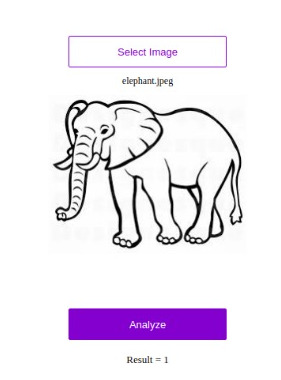
Zebra or Elephant?
This was exciting and fun. But I wanted to share the result, and my peer group aren’t all that familiar with log-loss scores. How could I get the point across and communicate what this means? Time to deploy this model as a web application 🙂
Exporting the model for later use
Final training step, saving weights and exporting to a file in my Google Drive
I knew it was possible to save some of the model parameters with model.save(‘name’), but wasn’t sure how easy it would be to get a complete model definition. Turns out, enough people want this that you can simply call model.export(‘model_name’). So I set my model training again (I hadn’t saved last time) and started researching my next step while Google did my computing for me.
Packaging as an app
I expected this step to be rather laborious. I’d need to set up a basic app (planned to use Flask), get an environment with pytorch/fastai set up and deploy to a server or, just maybe, get it going on Heroku. But then I came across an exciting page in the fastai docs: ‘Deploying on Render‘. There are essentially 3 steps: – Fork the example repository – Edit the file to add a link to your exported model – Sign up with Render and point it at your new GitHub repository. Then hit deploy! You can read about the full process in the aforementioned tutorial. Make sure your fastai is a recent version, and that you export the model (not just saving weights).
The resultant app is available at zebra-vs-elephant.onrender.com. I used an earlier model with 97% accuracy (since I’m enjoying that top spot on the leaderboard ;)) but it’s still surprisingly accurate. It even get’s cartoons right!
Please try it out and let me know what you think. It makes a best guess – see what it says for non-animals, or flatter your friends by classifying them as pachyderms.
Conclusion
There seems to be a theme to my last few posts: “Things that sound hard are now easy!”. It’s an amazing world we live in. You can make something like this! It took 20 minutes, with me doing setup while the model trained! Comment here with links to your sandwich-or-not website, your am-I-awake app, your ‘ask-a-computer-if-this-dolphin-looks-happy’ business idea. Who knows, one of us might even make something useful 🙂
Yes, that is apparently an elephant…
UPDATE: I’ve suspended the service for now, but can re-start it if you’d like to try it. Reach out if that’s the case 🙂
This week saw folks from all over the AI space converge in Cape Town for the AI Expo. The conference was inspiring, and I had a great time chatting to all sorts of interesting people. There were so many different things happening (which I’m not going to cover here), but the one that led to this post was a hackathon run by Zindi for their most recent Knowledge competition: the MIIA Pothole Image Classification Challenge. This post will cover the basic approach used by many entrants (thanks to Jan Marais’ excellent starting notebook) and how I improved on it with a few tweaks. Let’s dive in.
The Challenge
The dataset consists of images taken from behind the dashboard of a car. Some images contain potholes, some don’t – the goal is to correctly discern between the two classes. Some example pictures:
Train and test data were collected on different days, and at first glance it looks like this will be a tough challenge! It looks like the camera is sometimes at different angles (maybe to get a better view of potholes) and the lighting changes from pic to pic.
The first solution
Jan won a previous iteration of this hackathon, and was kind enough to share a starting notebook (available here) with code to get up and running. You can view the notebook for the full code, but the steps are both simple and incredibly powerful:
Load the data into a ‘databunch’, containing both the labeled training data and the unlabeled test data. Using 15% of the training data as a validation set. The images are scaled to 224px squares and grouped into batches.
The images are automatically warped randomly each time (to make the model more robust). This can be configured, but the default is pretty good.
Create a model: learn = cnn_learner(data, resnet18, metrics=accuracy). This single line does a lot! It downloads a pre-trained network (resnet18) that has already been optimised for image classification. It reconfigures the output of that network to match the number of classes in our problem. It links the model to the data, freezes the weights of the internal layers, and gives us a model ready for re-training on our own classes.
Pick a learning rate, by calling learn.lr_find() followed by learn.recorder.plot() and picking one just before the graph bottoms out (OK, it’s more complicated than that but you can learn the arcane art of lr optimization elsewhere)
*sucks thumb* A learning rate of 0.05 looks fine to me Bob.
Fit the model with learn.fit_one_cycle(3, lr) (Change number of epochs from 3 to taste), make predictions, submit!
There is some extra glue code to format things correctly, find the data and so on. But this is in essence a full image classification workflow, in a deceptively easy package. Following the notebook results in a log-loss score of ~0.56, which was on par with the top few entries on the leaderboard at the start of the hackathon. In the starter notebook Jan gave some suggestions for ways to improve, and it looks like the winners tried a few of those. The best score of the day was Ivor (Congrats!!) with a log-loss of 0.46. Prizes were won, fun was had and we all learned how easy it can be to build an image classifier by standing on the shoulders of giants.
Making it better
As the day kicked off, I dropped a few hints about taking a look at the images themselves and seeing how one could get rid of unnecessary information. An obvious answer would be to crop the images a little – there aren’t potholes in the dashboard or the sky! I don’t think anyone tried it, so let’s give it a go now and see where we get. One StackOverflow page later, I had code to crop and warp an image:
Before and after warping. Now the road is the focus, and we’re not wasting effort on the periphery.
I ran my code to warp all the images and store them in a new folder. Then I basically re-ran Jan’s starting notebook using the warped images (scaled to 200×200), trained for 5 epochs with a learning rate of 0.1, made predictions and…. 0.367 – straight to the top of the leader-board. The image warping and training took 1.5 hours on my poor little laptop CPU, which sort of limits how much iterating I’m willing to do. Fortunately, Google Colab gives a free GPU, cutting that time to a few minutes.
Conclusions
My time in the sun
Thanks to Google’s compute, it didn’t take long to have an even better model. I leave it to you dear readers to figure out what tweaks you’ll need to hop into that top spot.
My key takeaway from this is how easy it’s become to do this sort of thing. The other day I found code from 2014 where I was trying to spot things in an image with a kludged-together neural network. The difference between that and today’s exercise, using a network trained on millions of images and adapting it with ease thanks to a cool library and a great starting point… it just blows my mind how much progress has been made.
Why are you still reading this? Go enter the competition already! 🙂
Some students had asked me for my opinion on automated tools for machine learning. The thought occurred that I hadn’t done much with them recently, and it was about time I gave the much-hyped time savers a go – after all, aren’t they going to make data scientists like me redundant?
In today’s post, I’ll be trying out Google’s AutoML tool by throwing various datasets at it and seeing how well it does. To make things interesting, the datasets I’ll be using will be from Zindi competitions, letting us see where AutoML would rank on the player leader-board. I should note that these experiments are a learning exercise, and actually using AutoML to win contests is almost certainly against the rules. But with that caveat out the way, let’s get started!
How it works
AutoML (and other similar tools) aims to automate one step of the ML pipeline – that of model selection and tuning. You give it a dataset to work on, specify column types, choose an output column and specify how long you’d like it to train for (you pay per hour). Then sit back and wait. Behind the scenes, AutoML tries many different models and slowly optimizes network architecture, parameters, weights… essentially everything one could possibly tweak to improve performance gets tweaked. At the end of it, you get a (very complicated) model that you can then deploy with their services or use to make batch predictions.
The first step with AutoML tables – Importing the data.
The resultant models are fairly complex (mine were ~1GB each fully trained) and are not something you can simply download and use locally – you must deploy them via Google (for an extra fee). This, coupled with the cost of training models, makes it fairly expensive to experiment with if you use up your trial credits – so use them wisely.
Fortunately, there are other ways to achieve broadly the same result. For example, AutoKeras. Read more about that here.
Experiment 1: Farm Pin Crop Detection
This competition involves a classification problem, with the goal being to predict which crop is present in a given field. The training data is provided as field outlines and satellite images – not something that can effortlessly slot into AutoML tables. This meant that the first step was to sample the image bands for the different fields, and export the values to a CSV files for later analysis (as described in this post). This done, I uploaded the resultant training file to cloud storage, selected the table, chose my input and output columns and hit go.
AutoML ‘Evaluate’ tab showing model performance.
The scoring metric for this competition is log loss. My previous best (using the same training data to train a random forest model) scored around 0.64 (~20th on the leaderboard). So a score of <0.6 looked promising. I uploaded the test set, hit predict and then manually cleaned up the output to match the submission format for Zindi. Score? 0.546, putting me in 12th place. No feature engineering besides sampling some satellite images, no manual tweaking of model parameters…. not bad!
I was quite pleased with this result. I enjoy the feature engineering side of things, but the tedium of hyper-parameter tuning is less appealing to me. If this tool can magically let me skip that step, it’s a win in my book! I may re-visit this with some added features, information from more images and perhaps a trick or two to enlarge the training set.
Experiment 2: Traffic Jam
Spurred on by the first success, I turned to the Traffic Jam competition since I still had the dataset on my laptop. This was a regression problem, with the goal being to predict the number of tickets sold for a given trip into Nairobi. The training data was fairly sparse, with only ~2000 rows to work from. Still, I figured it was worth a shot and threw a few node hours worth of Google-managed ML magic at the problem.
An MAE of 3.4, hypothetically equivalent to ~3rd place!
The evaluation results had me excited – and MAE of 3.4 would have placed the model in third place had the competition remained open. I hastily uploaded the predictions to Zindi, to see the score of… 5.3 (160th place). Now, I might be missing some glaring error in the way I formatted predictions for upload, but I suspect that the issue is with AutoML. It’s not really designed for such small datasets. From the website: “Depending on how many features your dataset has, 1,000 rows might not be enough to train a high-performing model.” The impressive MAE shown in the results tab is for one particular test set, and it seems that for the Zindi test set we were simply not as lucky. Another potential factor: The random test set will have sampled from the same date range as the training data, whereas the Zindi test set was for a different time period. In cases like this, a non-shuffled test/train split can be a better indicator of true performance.
So, we’ve learnt something new! The magic tool isn’t magic, and just like any other method it needs good training data to make good predictions.
Experiment 3: Sendy
I couldn’t resist trying it out once more on the newly launched Sendy Competition. I merged the Riders info into the train and test sets, uploaded the data, gave it an hour of training time and set it going. The goal is to minimize RMSE when predicting travel time between two locations (for deliveries). I also did some modelling myself while I waited for the AutoML training to finish.
Scores (RMSE for predicted time in seconds) My first attempt (Catboost on provided data): 734 (7th place when this post was written) First place: 721 Google AutoML: 724 (4th place until I convince them to remove my latest entry)
Not too shabby! To me, one of the great uses of a tool like this is to give a ballpark for what a good model looks like. Without the Zindi leaderboard, I wouldn’t have a way to gauge my model performance. Is it good? Could it get better with the same data? Now I can compare to the AutoML, using it as a ‘probably close to best’ measure.
Where next?
These quick tests have convinced me that these automated tools can be a useful part of my workflow, but are not a complete replacement for manual experimentation, exploration, feature engineering and modelling. I intend to play around more with AutoML and other tools in the near future, so stay tuned for a continuation of this series.
In Part 1, I showed a quick way to get a model that predicts cropland extent, using someone else’s model as a starting point. This was a fun exercise, but in today’s post I’d like to show a more conventional approach to achieve the same goal, and then use that to track change in land cover over time within a region.
Training Data
This time, we’ll generate training data manually. For convenience, I’m changing the goalposts slightly: in this post, we’ll be making a simple model to distinguish between open land (fields, grassland, bare earth) and woodland. In the area of interest, this pretty much covers all the bases. Collecting data is a simple but laborious process – examples of each class are outlines in Google Earth Engine and saved as two separate FeatureCollections:
Some open areas (red) and woodland (green) manually outlined for training.
Modelling
We’ve covered modelling in GEE before, so I won’t go into details here. Sentinel 2 imagery is used, and I pretty much followed the docs to create a classifier and then apply it to the input image over the whole area. The model is fairly accurate, and a quick visual double-check confirms that it’s doing a good job of making the open areas:
Open area masked (left) vs input image (right)
Change over time
By choosing fields and wooded areas for training that have been present for decades, we can use the same training data to build models on imagery from different years. To track change in open land area, we can make a prediction for each year and sum the area that is classified as ‘open land’ with the following code snippet:
Getting the total area classified as open land over an ROI (ward 8)
For my ROI, the total open land trends steadily upwards. For dates earlier than 2015, I used Lnadsat 7 imagery as the input. From 2015 to 2018, Sentinel 2 Imagery was used as well as Landsat for comparison. In some years (2010 and 2018/19) there were enough cloudy images that I combined two years for the estimate. Some of the Landsat 7 imagery isn’t the best quality, and there are some issues with this approach that mean I wouldn’t trust the figures to be incredibly accurate. BUT, we’ve accomplished our goal: the figures show the change in land cover over time:
Conclusion
I hope this inspires you to try something like this for yourself, in an area that you’re interested in. I don’t think I’ll come back to this topic, although I’ll keep working on this project to turn it into something reliable (adding more training data, properly assessing accuracy, incorporating ground-truth data to verify etc etc). This post also marks the end of the Pioneer project mentioned here. My posting schedule will likely slow down, and you can expect some more diverse posts in the near future. Stay tuned!